
AI on Your Computer: Run a Local LLM Like a Service
Run a local LLM on macOS, Linux, or Windows, call it over HTTP like a real service, stream output in Node/Python/Go/C++, and measure TTFT + throughput to understand what's actually happening.
The day your "AI understanding" becomes real
Most explanations of AI feel like fog because they live at the wrong altitude. They float above the messy world where computers have fans, memory limits, and processes you can kill when they get weird. Developers do not build intuition from vocabulary; we build it from behavior. When you run a model locally, you stop believing in AI and start observing it. That shift replaces mysticism with mechanics, which is where learning gets fun. So we are going to drag the model down to the desk and watch it behave.
The practical milestone is treating a model like a service you would ship. A service has a port, an endpoint, real latency, and failure modes you can reproduce. A service can be called from Node today and Go tomorrow, and it still behaves like itself. A service can be measured, which means you can stop guessing about performance and start collecting receipts. By the end of this article, you will have that kind of service running on your own machine. That is the baseline we build from today.
What we're building today
Today's deliverable is intentionally boring in the best way: a local LLM that looks like any other backend dependency. You will start a runtime that exposes an HTTP API and talk to it from multiple languages. You will stream output so you can see the incremental nature of generation instead of imagining it. You will measure time-to-first-token (TTFT) and a simple throughput proxy so performance becomes tangible. Once those numbers exist, AI speed stops being a vibe and becomes a graphable property. With that baseline in place, the rest of the series can climb without hand-waving.
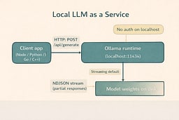
Under the hood, Ollama serves its API locally by default and is designed to be called like a normal web service. The base URL is http://localhost:11434/api, and endpoints like /api/generate stream responses by default. This is not a special AI protocol; it is HTTP with newline-delimited JSON (NDJSON), which means your existing engineering instincts apply. The key detail is that streaming makes TTFT visible, which is exactly what users feel. That makes the system measurable instead of mystical. With that contract in place, we can treat everything else as normal I/O and parsing.
The service boundary, explained
Transformers are the latest link in a chain that started with symbolic AI. The Dartmouth proposal in 1956 coined the field and framed intelligence as something that could be described precisely enough to implement in software.5 Early systems like ELIZA showed how far symbolic pattern matching could go without true understanding, which made the promise feel both exciting and fragile.6 Expert systems translated human judgment into rules, but the rule explosion made maintenance and coverage collapse under real-world complexity. The first AI winter arrived when ambitious programs failed to scale the rule-based approach. That failure pushed the field toward learning from data instead of encoding rules.
Statistical learning and neural nets rebuilt AI around data and gradients. Backpropagation proved that multi-layer networks could learn complex representations, which reopened the door to neural architectures at scale.7 Convolutional nets like LeNet showed that learned features could outperform hand-engineered ones, but compute and dataset size kept the wins narrow.8 The ImageNet benchmark finally supplied the data scale deep learning needed, and it became the proving ground for larger models.9 AlexNet’s 2012 result made the scale argument undeniable and pulled the industry into the deep learning era.10 Once scale worked for vision, language needed a way to handle long sequences efficiently.
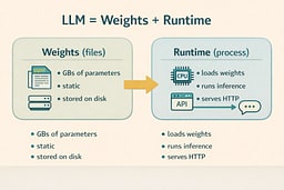
Attention removed the sequential bottleneck and made scale practical. Bahdanau attention let models focus on relevant input spans without forcing all context through a single bottleneck vector.11 The Transformer architecture eliminated recurrence and turned attention into a fully parallelizable core, which unlocked far larger training runs.12 BERT demonstrated that pretraining a transformer on large corpora produced reusable representations, and GPT-3 showed that sheer scale could unlock new behaviors without task-specific fine-tuning.13 14 Those breakthroughs are why a local model now looks like weights plus a runtime and why we care about the service boundary. With that lineage in mind, the rest of the article stays grounded in mechanics.
Choose your setup (macOS, Linux, Windows)
We're standardizing on Ollama so the runtime behaves consistently across operating systems and across the whole series. Ollama exposes a stable local API, serves it at a predictable address, and does not require authentication when you are hitting localhost.1 2 That is exactly what you want for learning, benchmarking, and building little local tools that behave like production services. Once you are running, the same client code works everywhere, which keeps your attention on concepts instead of OS trivia. The goal is to make the runtime boring so the behavior becomes obvious. Pick your OS and get to a running service.
Use the setup pages as a checklist and return here when the endpoint responds. On macOS, follow Local AI Lab Setup: macOS (Ollama) and pay attention to the macOS version requirement. On Linux, follow Local AI Lab Setup: Linux (Ollama) where you will likely run Ollama as a system service. On Windows, follow Local AI Lab Setup: Windows (Ollama) with the WSL2 path for Linux parity. If you want Ollama available on your local network, use Local AI Lab Setup: Docker (Ollama). Each path ends with the same result: a local HTTP service you can call. When your service answers HTTP requests, come back and we will start measuring reality.
Make sure the service answers before you optimize anything
Before you write a single line of client code, verify the server is reachable. Ollama serves its API locally, and the default base address is http://localhost:11434/api.1 That address is your contract: if it responds, the rest of your work becomes straightforward I/O and parsing. If it does not respond, you do not have an AI problem; you have a service management problem, which is refreshingly familiar. This mindset keeps you from debugging the wrong layer. If the endpoint responds, you are done with setup.
Ollama's local API does not require authentication when accessed via localhost, which keeps the learning loop fast and frictionless.2 Authentication shows up when you start using cloud models, publishing models, or downloading private models, but we are not doing any of that today. The point is to keep everything local, observable, and under your control. That is how you build a clean mental model. Stay local and keep it observable for now.
Pull a model and sanity-check inference
A runtime without weights is like Docker without images: technically installed, practically useless. Pull a small model first so you can iterate quickly and avoid waiting your way into boredom. Then run it interactively one time to confirm inference works end-to-end. The first run often feels slower because you are paying cold-start costs like loading weights into memory. Once that completes, subsequent runs usually speed up, which is a real-world performance lesson hiding in plain sight. When the interactive run responds, you know inference is alive.
ollama list
ollama pull llama3.2
ollama run llama3.2
When that interactive session produces a response, you have proven the whole stack works: storage, runtime, and inference. Now we can treat it like a service, because it is one. The rest of this article is simply learning to speak to it over HTTP and observing what happens when the system streams output under load. The moment you can drive it from curl, you have a real baseline. Next, we make that baseline visible on the wire.
Your local LLM is an HTTP API (and that's the best news you'll hear all week)
Ollama's /api/generate endpoint is the workhorse for single-turn text generation, and it supports streaming output by default.1 Streaming responses are delivered as NDJSON, which means your client receives a sequence of JSON objects rather than one giant blob.3 This is exactly how you want a responsive app to behave: TTFT can be low even when the full completion takes longer, and the user perceives that as fast. The behavior is not mystical; it is incremental output over a long-lived HTTP response. That is the same pattern used in many real-time systems. We will start by watching it directly.
If you want a single JSON response instead, you can disable streaming by sending "stream": false.1 That returns standard application/json, which is convenient for simple scripts and test harnesses. Both modes are useful, and you should get comfortable with both because real systems frequently offer the same tradeoff: easier parsing versus better perceived responsiveness. We are going to use streaming as the default because it teaches you more, faster. Once you see both modes, the service contract becomes obvious. Now let's watch the wire.
First request (curl): watch the wire, learn the truth
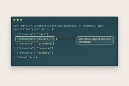
Start with curl because it is honest and has no opinions. A streaming request returns NDJSON lines, and each line is a small JSON object that may include a partial response field plus a done flag when generation finishes.1 3 Seeing this live is the moment many people finally understand token streaming as an engineering problem rather than a vibe. It is just line-delimited JSON over HTTP. The biggest lesson is that you are not waiting for a final blob. Run this and watch the output arrive line by line.
curl http://localhost:11434/api/generate \
  -H "Content-Type: application/json" \
  -d '{
    "model": "llama3.2",
    "prompt": "Explain what an LLM runtime is in one crisp paragraph for a software engineer."
  }'
Non-streaming mode is useful when you want one JSON payload with the final result. Streaming can be disabled by sending "stream": false, and Ollama will return a single response object instead of NDJSON lines. This is perfect for quick sanity checks and tiny automation scripts where you do not care about incremental output. Both modes are valid; they just optimize for different needs. Use this mode if you want a quick snapshot of the full completion. Once you have seen both, the interface feels familiar.
curl http://localhost:11434/api/generate \
  -H "Content-Type: application/json" \
  -d '{
    "model": "llama3.2",
    "prompt": "Give me 3 bullet points on what a model runtime does.",
    "stream": false
  }'
The streaming mental model (no mysticism, just plumbing)
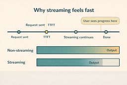
Streaming means the server sends partial output as it becomes available and the client consumes it incrementally. The magic feeling comes from the user seeing progress early, which is mostly a TTFT story. A low TTFT makes a system feel snappy even if the total completion time has not improved. This is why chat interfaces feel faster than submit-and-wait forms even when they cost the same compute. Streaming changes perception by changing the timing of feedback. That is the trick, and it is a plain engineering tradeoff.
NDJSON is simply a convenient envelope for that behavior. Each line is a self-contained JSON object, so clients can parse line by line without waiting for the full response.3 The engineering implications are familiar: you need buffering, newline splitting, and careful handling of partial data. The only AI-specific part is what the text means; the transport is plain old web plumbing. Once you understand that, you can implement clients in any language. Now we will do exactly that.
Working demo: Node.js streaming client (no dependencies)
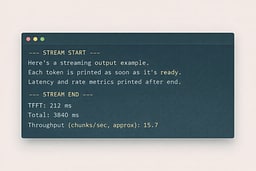
This Node script reads an NDJSON stream, prints partial output immediately, and measures TTFT plus a simple throughput proxy. The throughput here is chunks per second, not true tokenizer tokens, because our goal is to build intuition before chasing precision. The script is intentionally dependency-free so you can run it anywhere Node runs. The code uses the Fetch API, a readable stream, and a small line buffer. It is all standard web I/O. Save it as demo-node-stream.mjs and run it.
import { performance } from 'node:perf_hooks';

const url = 'http://localhost:11434/api/generate';
const body = {
  model: 'llama3.2',
  prompt:
    "Explain 'weights + runtime' like you're talking to a senior engineer who hates buzzwords.",
};

const start = performance.now();
let firstChunkAt = null;
let chunks = 0;

const res = await fetch(url, {
  method: 'POST',
  headers: { 'Content-Type': 'application/json' },
  body: JSON.stringify(body),
});

if (!res.ok) throw new Error(`HTTP ${res.status}: ${await res.text()}`);

const reader = res.body.getReader();
const decoder = new TextDecoder();
let buffer = '';

process.stdout.write('\n--- STREAM START ---\n\n');

while (true) {
  const { value, done } = await reader.read();
  if (done) break;

  buffer += decoder.decode(value, { stream: true });

  let idx;
  while ((idx = buffer.indexOf('\n')) >= 0) {
    const line = buffer.slice(0, idx).trim();
    buffer = buffer.slice(idx + 1);
    if (!line) continue;

    const msg = JSON.parse(line);

    if (msg.response) {
      if (firstChunkAt === null) firstChunkAt = performance.now();
      chunks += 1;
      process.stdout.write(msg.response);
    }

    if (msg.done) {
      const end = performance.now();
      const ttftMs = firstChunkAt ? firstChunkAt - start : null;
      const totalMs = end - start;
      const cps = chunks / (totalMs / 1000);

      process.stdout.write('\n\n--- STREAM END ---\n');
      console.log(`TTFT: ${ttftMs?.toFixed(0)} ms`);
      console.log(`Total: ${totalMs.toFixed(0)} ms`);
      console.log(`Throughput (chunks/sec, approx): ${cps.toFixed(1)}`);
    }
  }
}
Run it and pay attention to TTFT versus total time. If TTFT is high, your model is likely cold, memory pressure is high, or the model is too large for your machine. If TTFT is low but total time is high, you have learned a key UX truth: streaming can make slow systems feel usable. The point is not to chase perfect numbers yet; the point is to stop guessing and start observing. Once you have that baseline, reproduce it in Python to make the pattern feel portable.
node demo-node-stream.mjs
Working demo: Python streaming client
The Python version uses requests in streaming mode and mirrors the same TTFT and chunk-rate measurements. This is a great template for quick CLIs, notebooks, or little AI utilities you want to wire into your workflow. It is also a reminder that the model does not care what language you prefer; the API contract stays the same. The script prints partial output as it arrives and then emits the timing summary. Save it as demo_python_stream.py and keep it in the same folder as your Node script.
import json
import time
import requests

URL = 'http://localhost:11434/api/generate'
payload = {
    'model': 'llama3.2',
    'prompt': 'Explain TTFT in one paragraph, practically.'
}

start = time.perf_counter()
first = None
chunks = 0

with requests.post(URL, json=payload, stream=True) as r:
    r.raise_for_status()
    for line in r.iter_lines():
        if not line:
            continue
        msg = json.loads(line.decode('utf-8'))

        if msg.get('response'):
            if first is None:
                first = time.perf_counter()
            chunks += 1
            print(msg['response'], end='', flush=True)

        if msg.get('done'):
            end = time.perf_counter()
            ttft_ms = (first - start) * 1000 if first else None
            total_ms = (end - start) * 1000
            cps = chunks / ((end - start) or 1)
            print('\n\n---')
            print(f'TTFT: {ttft_ms:.0f} ms' if ttft_ms else 'TTFT: n/a')
            print(f'Total: {total_ms:.0f} ms')
            print(f'Throughput (chunks/sec, approx): {cps:.1f}')
Install the dependency once and run the script. You are not looking for identical numbers; you are looking for consistent behavior across languages. When TTFT changes between runs, you are discovering caching and cold-start effects in the most hands-on way possible. The stream should look and feel the same as the Node run, because the API contract did not change. That is the point of a service boundary. Next, we will do the same thing in Go.
python3 -m pip install requests
python3 demo_python_stream.py
Working demo: Go streaming client (scanner buffer made safe)
Go is a great truth-serum language for streaming because it forces you to be explicit about buffering and parsing. This client reads NDJSON lines with a scanner, expands the default buffer to avoid pathological failures, and prints output as it arrives. The measurement logic again focuses on TTFT and a rough chunk rate because the goal is comparative intuition. The code is small but not magical, and that is exactly why it teaches well. Save it as demo_go_stream.go and run it locally.
package main

import (
  "bufio"
  "bytes"
  "encoding/json"
  "fmt"
  "net/http"
  "time"
)

type Line struct {
  Response string `json:"response"`
  Done     bool   `json:"done"`
}

func main() {
  url := "http://localhost:11434/api/generate"
  payload := []byte(`{"model":"llama3.2","prompt":"Explain a local LLM as if it were just another backend dependency."}`)

  start := time.Now()
  var first time.Time
  chunks := 0

  req, err := http.NewRequest("POST", url, bytes.NewReader(payload))
  if err != nil {
    panic(err)
  }
  req.Header.Set("Content-Type", "application/json")

  resp, err := http.DefaultClient.Do(req)
  if err != nil {
    panic(err)
  }
  defer resp.Body.Close()

  fmt.Println("\n--- STREAM START ---\n")

  sc := bufio.NewScanner(resp.Body)
  sc.Buffer(make([]byte, 0, 64*1024), 1024*1024)

  for sc.Scan() {
    line := bytes.TrimSpace(sc.Bytes())
    if len(line) == 0 {
      continue
    }

    var msg Line
    if err := json.Unmarshal(line, &msg); err != nil {
      panic(err)
    }

    if msg.Response != "" {
      if first.IsZero() {
        first = time.Now()
      }
      chunks++
      fmt.Print(msg.Response)
    }

    if msg.Done {
      fmt.Println("\n\n--- STREAM END ---")
      ttft := first.Sub(start)
      total := time.Since(start)
      cps := float64(chunks) / total.Seconds()
      fmt.Printf("TTFT: %d ms\n", ttft.Milliseconds())
      fmt.Printf("Total: %d ms\n", total.Milliseconds())
      fmt.Printf("Throughput (chunks/sec, approx): %.1f\n", cps)
    }
  }

  if err := sc.Err(); err != nil {
    panic(err)
  }
}
Run it and compare the shape of the stream to the other languages. You are building a transferable model: a local service streams NDJSON lines, clients parse and print, and measurement wraps the call to quantify experience. Once that is internalized, adding token-accurate throughput later is a refinement, not a conceptual leap. The details may differ, but the behavior should match. Next, we will strip it down even further with C++ and libcurl.
go run demo_go_stream.go
Working demo: C++ streaming client (libcurl)
C++ is the down-to-the-metal view that proves the point: this is just HTTP and bytes. We use libcurl with a write callback, buffer partial chunks, split on newlines, and print each NDJSON line as it arrives. This version prints raw JSON lines rather than extracting only the response field because it is meant to reveal the wire format clearly. The code is deliberately minimal so the streaming behavior is obvious. Save it as demo_cpp_stream.cpp and compile it with libcurl installed.
#include <curl/curl.h>
#include <iostream>
#include <string>

static size_t write_cb(char* ptr, size_t size, size_t nmemb, void* userdata) {
  auto* buffer = static_cast<std::string*>(userdata);
  buffer->append(ptr, size * nmemb);

  size_t pos = 0;
  while ((pos = buffer->find('\n')) != std::string::npos) {
    std::string line = buffer->substr(0, pos);
    buffer->erase(0, pos + 1);
    if (!line.empty()) std::cout << line << std::endl;
  }
  return size * nmemb;
}

int main() {
  CURL* curl = curl_easy_init();
  if (!curl) return 1;

  const char* url = "http://localhost:11434/api/generate";
  std::string payload =
      R"({"model":"llama3.2","prompt":"Explain local LLMs like you're explaining Docker to a friend."})";

  struct curl_slist* headers = nullptr;
  headers = curl_slist_append(headers, "Content-Type: application/json");

  std::string buffer;

  curl_easy_setopt(curl, CURLOPT_URL, url);
  curl_easy_setopt(curl, CURLOPT_HTTPHEADER, headers);
  curl_easy_setopt(curl, CURLOPT_POSTFIELDS, payload.c_str());
  curl_easy_setopt(curl, CURLOPT_WRITEFUNCTION, write_cb);
  curl_easy_setopt(curl, CURLOPT_WRITEDATA, &buffer);

  CURLcode res = curl_easy_perform(curl);
  if (res != CURLE_OK) {
    std::cerr << "curl error: " << curl_easy_strerror(res) << "\n";
  }

  curl_slist_free_all(headers);
  curl_easy_cleanup(curl);
  return 0;
}
Build steps vary by OS, so install libcurl with your package manager and compile using your platform's include and library paths (see the setup pages for OS-specific commands). If pkg-config is available, it is the simplest cross-platform way to wire in the flags. The core learning is that a model service is not a magical SDK; it is a process that speaks HTTP and streams JSON lines. Once that is true, every language can be a client. That is exactly the service boundary we want.
c++ demo_cpp_stream.cpp -o demo_cpp_stream $(pkg-config --cflags --libs libcurl)
./demo_cpp_stream
Real-world guidance (the stuff that matters after the demo works)
Streaming makes apps feel fast because humans measure waiting, not compute
People perceive systems through feedback timing, not through total runtime. If TTFT is low, users feel like the system is responsive, even if the full completion still takes time. Streaming also keeps UI event loops alive because you can render partial output while generation continues. This is why chat interfaces feel faster than batch-style responses even when they are not cheaper. The lesson is not that streaming makes compute cheaper; it makes experience better. When you build products with local models, streaming is the difference between "this is neat" and "this is usable."
Model size is physics wearing a trench coat
Bigger models mean more memory pressure, more bandwidth to load weights, and more math per generated token. On constrained machines, large models can look like they are thinking hard when they are really just paging memory and running out of cache. Start small so you can build your harness quickly and then scale up when your measurement loop is stable. Treat model choice like a performance budget decision, not a philosophical identity. If you want your laptop to stay a laptop, pick models that fit your hardware reality.
Reliability still matters, even when the server is just your computer
A local model is still a dependency, and dependencies deserve guardrails. Put timeouts around calls so a stuck generation does not freeze your app. Support cancellation so users can stop a runaway response without waiting for the server to finish its dramatic monologue. Use retries only when they make sense, and keep them bounded so you do not amplify load. The takeaway is simple: the moment you treat the model like a service, you should also treat it like a service operationally. That is the difference between a demo and a tool you trust.
Our throughput number is intentionally approximate (for now)
We measured chunks per second because it is easy, observable, and good enough to build intuition. True token throughput depends on tokenizer specifics and sampling settings, and we will get there soon. The next article will add token counting and show how sampling parameters change speed and output quality. Today's job is to build the baseline: a working service, a streaming client, and metrics you can reproduce. Precision is a sequel; intuition is the first draft.
Optional: OpenAI-style endpoints with llama.cpp (a compatibility escape hatch)
Some toolchains expect OpenAI-shaped endpoints like /v1/chat/completions, and some older machines cannot run newer runtimes. This is where llama.cpp and its llama-server can be useful, because it can expose OpenAI-compatible routes while still running locally.4 This path is especially relevant if you are on an older macOS version that cannot meet Ollama's requirements or if you want to test OpenAI-style payloads locally without rewriting clients. Consider it the adapter plug in your local AI lab. The service contract stays familiar even when the runtime changes.
We are not switching the series over today because consistency matters more than novelty. However, it is worth knowing this option exists so you do not get stuck on one runtime. In later parts of the series, we will cover tokenizer-accurate throughput and sampling controls, and that is the natural place to introduce alternate runtimes. For now, the goal is to master one service contract and make it boringly dependable. Once it is boring, you can build on it forever.
The service boundary is now real
You now have the only mental model that matters: a local LLM is just a service with weights behind it. You installed a runtime, pulled weights, verified the endpoint, and streamed output in multiple languages. You measured TTFT and a rough throughput proxy, which turns hand-wavy performance talk into something you can observe and compare. That small loop of request, stream, and measurement is the foundation for every optimization and product decision you will make later. Next, we will make the numbers more precise by counting real tokens and exploring how sampling choices bend both speed and output quality.
Sources
[2] Ollama FAQ
[4] llama.cpp repository (server example in README)
[5] Dartmouth Summer Research Project on Artificial Intelligence (1956 proposal)
[6] Weizenbaum, J. (1966). ELIZA: A Computer Program for the Study of Natural Language Communication
[7] Rumelhart, Hinton, Williams (1986). Learning representations by back-propagating errors
[8] LeCun et al. (1998). Gradient-based learning applied to document recognition (LeNet)
[9] Deng et al. (2009). ImageNet: A large-scale hierarchical image database
[10] Krizhevsky, Sutskever, Hinton (2012). ImageNet Classification with Deep Convolutional Neural Networks (AlexNet)
[11] Bahdanau, Cho, Bengio (2014). Neural Machine Translation by Jointly Learning to Align and Translate
[12] Vaswani et al. (2017). Attention Is All You Need
[13] Devlin et al. (2018). BERT: Pre-training of Deep Bidirectional Transformers
[14] Brown et al. (2020). Language Models are Few-Shot Learners (GPT-3)

About Joshua Morris
Joshua is a software engineer focused on building practical systems and explaining complex ideas clearly.