Insertion Sort: Building Order One Element at a Time

The Night My Kids Cleaned Their Rooms Without Fighting

There was a night—an unusual, shimmering, statistically improbable night—when all three of my kids decided to clean their rooms without arguing, bargaining, forming coalitions, or engaging in minor geopolitical maneuvers over toy ownership. They each picked up a single item, looked for where it belonged, and placed it there. One object. One position. Then the next object. No “dump everything out and start over,” no grand reshuffling, just incremental progress toward a clean floor.

That’s Insertion Sort.

It doesn't transform the whole array at once. It doesn't make sweeping, dramatic reorganizations. Instead, it looks at one element, finds the correct place for it, and gently slides it into order. It's calm, predictable, and profoundly human—the way we naturally organize things.

What Sorting Really Means

Sorting is less about "making everything ordered" and more about transforming chaos into a structure that supports fast lookup, predictable performance, and meaningful organization. In the Algorithm Series, each sorting algorithm reflects a different philosophy:

• Bubble Sort nudges neighbors into harmony through adjacent swaps.
• Merge Sort works by carefully orchestrating divide-and-conquer.
• Quick Sort relies on clever partitioning around pivots.
• Insertion Sort, the star of today's article, sorts the way we do with our own hands.

If Bubble Sort is the gentle simmer, Insertion Sort is the steady hand making small, deliberate fixes until everything settles into place.

Why Insertion Sort Exists

Insertion Sort fills a niche that no other simple algorithm handles as gracefully:
It is the champion of small, nearly sorted, and incrementally built lists.

Its core idea is simple:

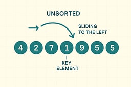
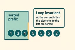
1. The left portion of the list is always sorted.
2. Each new element is inserted into this sorted prefix.
3. Move left until the new element fits.

This makes Insertion Sort:

• Stable
• Predictable
• Easy to reason about
• Ideal for systems where data arrives one item at a time

And because of its tight inner loop and excellent cache behavior, Insertion Sort can outperform more “advanced” algorithms on small datasets where constant factors dominate.

Credit: MethodicalFunction.com.

A Walkthrough You Can See

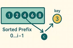
Insertion Sort works by maintaining a sorted prefix and inserting each new element into its correct position. The algorithm processes elements one at a time, comparing each new element with the sorted portion and shifting elements right until the correct insertion point is found. This approach ensures that after each iteration, the prefix remains sorted, building the final sorted array incrementally. The process is deterministic, stable, and requires no additional memory beyond the input array itself. Understanding this step-by-step process makes the algorithm's correctness and efficiency clear.

Consider the list:

[5, 2, 4, 6, 1, 3]

We start with i = 1, which means we begin processing from the second element. The first element (5) is already considered part of the sorted prefix, even though it's just one element. The key element at index 1 is 2, which we need to insert into the sorted prefix. We compare 2 with 5, and since 2 < 5, we shift 5 one position to the right. This creates space at index 0, where we insert 2. The sorted prefix now contains two elements: [2, 5], and the rest of the array remains unchanged.

Now the prefix is sorted:

[2, 5, 4, 6, 1, 3]

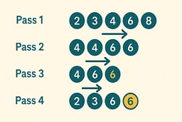
We continue with i = 2, where the key is 4. We compare 4 with 5 and find that 4 < 5, so we shift 5 right. We then compare 4 with 2 and find that 4 > 2, so we stop shifting and insert 4 at index 1. The sorted prefix grows to three elements: [2, 4, 5]. This process continues for each remaining element, with each insertion maintaining the sorted property of the prefix.

One element at a time, the sorted region grows—always correct, always stable. The algorithm's beauty lies in its simplicity: each insertion is independent, and the invariant guarantees correctness at every step.

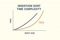
Complexity: Why O(n²) Isn't Always Bad

Insertion Sort has a reputation problem—it's "quadratic," and therefore assumed slow. But that ignores a key truth: real-world data is often almost sorted. The algorithm's performance characteristics reveal why it remains relevant despite its theoretical complexity. In the best case, when data is already sorted, Insertion Sort runs in linear time O(n), making only n-1 comparisons and zero shifts. The average case requires O(n²) operations, but with a smaller constant factor than many other quadratic algorithms. The worst case occurs with reverse-sorted data, requiring O(n²) comparisons and shifts. Space complexity is constant O(1), as the algorithm sorts in place without requiring additional memory structures. The algorithm is stable, preserving the relative order of equal elements, which is crucial for many real-world applications.

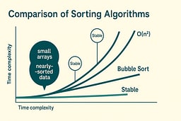
When the list is nearly sorted, Insertion Sort performs exceptionally well. Each new element requires only a few comparisons to find its position, and the number of shifts is minimal. This adaptive behavior makes Insertion Sort faster than algorithms with better worst-case complexity when dealing with partially ordered data. The algorithm's tight inner loop and excellent cache locality contribute to its practical efficiency. Modern processors benefit from the sequential memory access patterns that Insertion Sort exhibits, reducing cache misses and improving real-world performance.

Insertion Sort thrives in cases where Bubble Sort struggles: fewer swaps, fewer redundant comparisons, and faster convergence on nearly sorted data. The algorithm's ability to recognize and exploit existing order in the input makes it a valuable tool in the programmer's toolkit, despite its quadratic worst-case complexity.

Credit: MethodicalFunction.com.

Where Insertion Sort Wins in Real Life

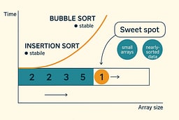
Real systems rarely hand you completely random data. Instead, you get logs that are already roughly chronological, UI lists where only one or two items changed, sensor data arriving sequentially, "just append and maintain sorted order" workloads, and batches of small arrays that must be sorted frequently. These common scenarios play to Insertion Sort's strengths, making it more practical than theoretical analysis might suggest. The algorithm's adaptive nature means it performs best when the input is partially ordered, which is the norm rather than the exception in production systems. Understanding where Insertion Sort excels helps developers make informed decisions about algorithm selection.

Insertion Sort dominates when arrays are smaller than approximately 50 elements, when data is almost sorted, when elements arrive one at a time, when cache locality matters, and when stability is required. The algorithm's simplicity and efficiency on small datasets make it the preferred choice for hybrid sorting algorithms that switch strategies based on input size. Its stable sorting property ensures that equal elements maintain their relative order, which is essential for maintaining data integrity in many applications. The algorithm's in-place nature and minimal memory overhead make it suitable for resource-constrained environments.

This is why Python's Timsort uses Insertion Sort internally for small runs, Java's Dual-Pivot Quicksort switches to Insertion Sort for small arrays, and C++'s standard library sorts also use it for tiny partitions. These production-grade sorting algorithms recognize Insertion Sort's practical advantages and incorporate it as a building block. It's the little algorithm that the big ones secretly rely on, proving that sometimes the simplest solution is the most effective.

Why We Naturally Use Insertion Sort

We sort like this intuitively when organizing papers, arranging books alphabetically, dealing cards, tidying a desk, and putting items in a shopping cart in a preferred order. These everyday activities demonstrate the natural approach to ordering: we maintain a sorted section and insert new items into their correct positions. This cognitive pattern makes Insertion Sort one of the most intuitive algorithms to understand and implement. The algorithm's behavior matches our mental model of sorting, making it easier to reason about correctness and performance.

Insertion Sort is effective because it mirrors cognitive ergonomics. We maintain a mental "sorted prefix" that represents the portion of the list we've already organized. We insert new items into this known order by finding the appropriate position through comparison. We rarely inspect the whole list—just what's needed to determine the insertion point. This focused approach reduces cognitive load and makes the algorithm's logic transparent. The algorithm's step-by-step nature allows us to verify correctness at each stage, building confidence in the implementation.

We don't bubble neighbors. We insert. This fundamental difference in approach explains why Insertion Sort feels more natural than Bubble Sort and why it performs better in practice. The algorithm's alignment with natural organizing cognitive patterns makes it an excellent teaching tool and a practical solution for many real-world sorting problems.

Comparing Insertion Sort to Bubble Sort

Insertion Sort

• Fewer swaps
• Fewer redundant comparisons
• Faster on nearly sorted data
• Uses shifting, not pairwise bubbling
• Grows a sorted prefix deliberately and consistently
• Much more useful in real applications

Bubble Sort

• Conceptually simpler
• Easy to visualize
• Intuitive for adjacent checks
• But extremely slow on anything beyond tiny input

Winner for real-world use:
Insertion Sort, every time.

Credit: MethodicalFunction.com.

Comparing Insertion Sort to Min/Max Scanning

Min/max scan algorithm:

• Finds an extreme value in O(n)
• Requires no reordering
• Teaches invariants and scanning fundamentals

Insertion Sort:

• Creates full sorted order
• Uses the same scanning idea internally
• Applies it repeatedly to build structure

Insertion Sort is essentially:
"Find where this belongs, then shift accordingly."

Credit: MethodicalFunction.com.

The Loop Invariant That Makes the Algorithm Work

The loop invariant is the mathematical property that guarantees Insertion Sort's correctness. At the start of each iteration i, the prefix a[0..i−1] is sorted. This invariant serves as a contract that the algorithm maintains throughout its execution, providing a foundation for proving correctness. The invariant is established before the loop begins, as a single-element array is trivially sorted. During each iteration, the algorithm preserves the invariant by inserting the current element into its correct position within the sorted prefix. The invariant ensures that after processing all elements, the entire array is sorted.

This invariant guarantees that the prefix is always correct, that inserting the next element preserves the sorted property, and that by the end, the entire list is sorted. The invariant's power lies in its simplicity: it states exactly what we need to know at each step, making the algorithm's correctness self-evident. When we insert an element, we shift larger elements to the right, maintaining the sorted order of the prefix. The insertion point is determined by comparing the key with elements in the sorted prefix, ensuring that all elements to the left of the insertion point are smaller than or equal to the key, and all elements to the right are larger.

Understanding the invariant makes the correctness proof trivial. We can verify that the invariant holds initially, that each iteration preserves it, and that termination guarantees the desired result. This mathematical rigor distinguishes well-designed algorithms from ad-hoc solutions, providing confidence in the implementation's correctness.

Credit: MethodicalFunction.com.

Pseudocode with Invariants

Credit: MethodicalFunction.com.

Algorithm InsertionSort(list)
    for i ← 1 to n−1 do
        key ← list[i]
        j ← i − 1

        while j ≥ 0 and list[j] > key do
            list[j+1] ← list[j]
            j ← j − 1
        end while

        list[j+1] ← key
    return list

Invariant: At the start of each iteration i, the prefix list[0..i−1] is sorted. After inserting key at position j+1, the prefix list[0..i] remains sorted.

I like this because the invariant is obvious: after processing each element, the sorted prefix grows by one, and the insertion process maintains the sorted property. The algorithm's correctness follows directly from the invariant's preservation 1.

How I write it in real languages

Now that we understand what Insertion Sort is and why its invariant matters, let's implement it in multiple languages to see how the same logic adapts to different ecosystems. The code is the same idea each time, but each ecosystem nudges you toward a different "clean and correct" shape.

When You'd Actually Use This

• Small datasets: When n < 50, Insertion Sort's simplicity and low overhead make it faster than more complex algorithms
• Nearly sorted data: When most elements are already in order, Insertion Sort's adaptive behavior shines
• Streaming data: When elements arrive one at a time and must be inserted into a sorted structure
• Hybrid algorithms: As a building block in Timsort, Introsort, and other adaptive sorting algorithms
• Educational purposes: Teaching invariants, correctness proofs, and algorithm design principles

Production note: For real applications with large, random datasets, use your language's built-in sort (typically O(n log n)) or a library implementation. Insertion Sort is a teaching tool and a component of hybrid algorithms, not typically a standalone production solution 3 6.

Why Study an Algorithm You'll Rarely Use Alone?

Why study an algorithm you'll rarely use alone in production? Because Insertion Sort teaches you to recognize when simplicity beats complexity. That small array in your hot path? Insertion Sort might be faster. That nearly-sorted data structure? Insertion Sort adapts beautifully. Understanding Insertion Sort's strengths makes you a better algorithm designer, even when you're using more sophisticated tools. It's the algorithm equivalent of understanding how a simple lever works—you might use a complex machine, but knowing the fundamentals makes you a better engineer.

C (C17): control everything, assume nothing

// insertion_sort.c
// Compile: cc -std=c17 -O2 -Wall -Wextra -o insertion_sort insertion_sort.c
// Run:     ./insertion_sort
#include <stdio.h>
#include <stddef.h>

void insertion_sort(int arr[], size_t n) {
    if (n == 0) return; // empty array is already sorted
    // Invariant: At the start of each iteration i, arr[0..i-1] is sorted
    for (size_t i = 1; i < n; i++) {
        int key = arr[i];
        size_t j = i;

        while (j > 0 && arr[j - 1] > key) {
            arr[j] = arr[j - 1];
            j--;
        }
        arr[j] = key;
    }
}

int main(void) {
    int a[] = {5, 2, 4, 6, 1, 3};
    size_t n = sizeof a / sizeof a[0];
    insertion_sort(a, n);
    for (size_t i = 0; i < n; i++) {
        printf("%d ", a[i]);
    }
    printf("\n");
    return 0;
}

C rewards paranoia. I guard against empty arrays, use size_t for indices to avoid signed/unsigned bugs, and keep the loop body tiny so the invariant stays visible. No heap allocations, no surprises.

C++20: let the standard library say the quiet part out loud

// insertion_sort.cpp
// Compile: c++ -std=c++20 -O2 -Wall -Wextra -o insertion_sort_cpp insertion_sort.cpp
// Run:     ./insertion_sort_cpp
#include <algorithm>
#include <array>
#include <iostream>

template<typename Iterator>
void insertion_sort(Iterator first, Iterator last) {
    if (first == last) return;
    // Invariant: At the start of each iteration, [first, current) is sorted
    for (auto it = std::next(first); it != last; ++it) {
        auto key = *it;
        auto j = it;

        while (j != first && *std::prev(j) > key) {
            *j = *std::prev(j);
            --j;
        }
        *j = key;
    }
}

int main() {
    std::array<int, 6> numbers{5, 2, 4, 6, 1, 3};
    insertion_sort(numbers.begin(), numbers.end());
    for (const auto& n : numbers) {
        std::cout << n << " ";
    }
    std::cout << "\n";
    return 0;
}

The iterator-based version works with any container. The template lets you sort anything comparable. In production, you'd use std::sort, but this shows the algorithm clearly 1 2.

Python 3.11+: readable first, but show your invariant

# insertion_sort.py
# Run: python3 insertion_sort.py
def insertion_sort(xs):
    """Sort list in-place using Insertion Sort."""
    xs = list(xs)  # Make a copy to avoid mutating input
    if not xs:
        return xs
    # Invariant: At the start of each iteration i, xs[0..i-1] is sorted
    for i in range(1, len(xs)):
        key = xs[i]
        j = i - 1

        while j >= 0 and xs[j] > key:
            xs[j+1] = xs[j]
            j -= 1

        xs[j+1] = key
    return xs

if __name__ == "__main__":
    numbers = [5, 2, 4, 6, 1, 3]
    result = insertion_sort(numbers)
    print(" ".join(map(str, result)))

Yes, sorted() exists. I like the explicit loop when teaching because it makes the invariant obvious and keeps the complexity discussion honest. For production code, use sorted() or list.sort().

Go 1.22+: nothing fancy, just fast and clear

// insertion_sort.go
// Build: go build -o insertion_sort_go ./insertion_sort.go
// Run:   ./insertion_sort_go
package main

import "fmt"

func InsertionSort(nums []int) []int {
	b := append([]int(nil), nums...) // Copy to avoid mutating input
	if len(b) == 0 {
		return b
	}
	// Invariant: At the start of each iteration i, b[0..i-1] is sorted
	for i := 1; i < len(b); i++ {
		key := b[i]
		j := i - 1
		for j >= 0 && b[j] > key {
			b[j+1] = b[j]
			j--
		}
		b[j+1] = key
	}
	return b
}

func main() {
	numbers := []int{5, 2, 4, 6, 1, 3}
	result := InsertionSort(numbers)
	fmt.Println(result)
}

Go code reads like you think. Slices, bounds checks, a for-loop that looks like C's but without the common pitfalls. The copy prevents mutation surprises, and the behavior is obvious at a glance.

Ruby 3.2+: expressiveness without losing the thread

# insertion_sort.rb
# Run: ruby insertion_sort.rb
def insertion_sort(arr)
  return arr if arr.empty?
  arr = arr.dup  # Copy to avoid mutating input
  # Invariant: At the start of each iteration i, arr[0..i-1] is sorted
  (1...arr.length).each do |i|
    key = arr[i]
    j = i - 1
    while j >= 0 && arr[j] > key
      arr[j+1] = arr[j]
      j -= 1
    end
    arr[j+1] = key
  end
  arr
end

numbers = [5, 2, 4, 6, 1, 3]
puts insertion_sort(numbers).join(" ")

It's tempting to use Array#sort, and you should in most app code. Here I keep the loop visible so the "insert and shift" pattern is easy to reason about. Ruby stays readable without hiding the algorithm.

JavaScript (Node ≥18 or the browser): explicit beats clever

// insertion_sort.mjs
// Run: node insertion_sort.mjs
function insertionSort(arr) {
  const a = arr.slice(); // Copy to avoid mutating input
  if (a.length === 0) return a;
  // Invariant: At the start of each iteration i, a[0..i-1] is sorted
  for (let i = 1; i < a.length; i++) {
    const key = a[i];
    let j = i - 1;

    while (j >= 0 && a[j] > key) {
      a[j + 1] = a[j];
      j--;
    }

    a[j + 1] = key;
  }
  return a;
}

const numbers = [5, 2, 4, 6, 1, 3];
console.log(insertionSort(numbers).join(' '));

Array.prototype.sort() is fine for production, but this shows the algorithm clearly. The explicit loop makes the invariant obvious, and the early termination prevents unnecessary comparisons.

React (tiny demo): compute, then render

// InsertionSortDemo.jsx
import { useState, useEffect } from 'react';

function insertionSortStep(arr, setState) {
  const a = [...arr];
  let i = 1;
  while (i < a.length && a[i] >= a[i - 1]) {
    i++;
  }
  if (i < a.length) {
    const key = a[i];
    let j = i - 1;
    while (j >= 0 && a[j] > key) {
      a[j + 1] = a[j];
      j--;
    }
    a[j + 1] = key;
    setState({ array: a, done: false });
  } else {
    setState({ array: a, done: true });
  }
}

export default function InsertionSortDemo({ list = [5, 2, 4, 6, 1, 3] }) {
  const [state, setState] = useState({ array: list, done: false });

  useEffect(() => {
    if (!state.done) {
      const timer = setTimeout(() => {
        insertionSortStep(state.array, setState);
      }, 300);
      return () => clearTimeout(timer);
    }
  }, [state]);

  return (
    <div>
      <p>{state.array.join(', ')}</p>
      {state.done && <p>Sorted!</p>}
    </div>
  );
}

In UI, you want clarity and visual feedback. This demo shows each insertion step, making the algorithm's progress visible. For production sorting, use Array.prototype.sort() or a library.

TypeScript 5.0+: types that document intent

// insertion_sort.ts
// Compile: tsc insertion_sort.ts
// Run:     node insertion_sort.js
export function insertionSort(arr: number[]): number[] {
  const a = arr.slice(); // Copy to avoid mutating input
  if (a.length === 0) return a;
  // Invariant: At the start of each iteration i, a[0..i-1] is sorted
  for (let i = 1; i < a.length; i++) {
    const key = a[i];
    let j = i - 1;

    while (j >= 0 && a[j] > key) {
      a[j + 1] = a[j];
      j--;
    }

    a[j + 1] = key;
  }
  return a;
}

const numbers = [5, 2, 4, 6, 1, 3];
console.log(insertionSort(numbers).join(' '));

// Generic version for any comparable type:
function insertionSortGeneric<T>(
  arr: T[],
  compare: (a: T, b: T) => number
): T[] {
  const a = arr.slice();
  if (a.length === 0) return a;
  for (let i = 1; i < a.length; i++) {
    const key = a[i];
    let j = i - 1;
    while (j >= 0 && compare(a[j], key) > 0) {
      a[j + 1] = a[j];
      j--;
    }
    a[j + 1] = key;
  }
  return a;
}

TypeScript's type system catches errors at compile time, and generics let you reuse the same logic for strings, dates, or custom objects with comparators.

Java 17+: enterprise-grade clarity

// InsertionSort.java
// Compile: javac InsertionSort.java
// Run:     java InsertionSort
public class InsertionSort {
    public static void insertionSort(int[] arr) {
        if (arr.length == 0) return;
        // Invariant: At the start of each iteration i, arr[0..i-1] is sorted
        for (int i = 1; i < arr.length; i++) {
            int key = arr[i];
            int j = i - 1;

            while (j >= 0 && arr[j] > key) {
                arr[j+1] = arr[j];
                j--;
            }
            arr[j+1] = key;
        }
    }

    public static void main(String[] args) {
        int[] numbers = {5, 2, 4, 6, 1, 3};
        insertionSort(numbers);
        for (int n : numbers) {
            System.out.print(n + " ");
        }
        System.out.println();
    }
}

Java's explicit types and checked exceptions make contracts clear. The JVM's JIT compiler optimizes the hot path, so this performs well in production.

Rust 1.70+: zero-cost abstractions with safety

// insertion_sort.rs
// Build: rustc insertion_sort.rs -o insertion_sort_rs
// Run:   ./insertion_sort_rs
fn insertion_sort(nums: &mut [i32]) {
    if nums.is_empty() {
        return;
    }
    // Invariant: At the start of each iteration i, nums[0..i-1] is sorted
    for i in 1..nums.len() {
        let key = nums[i];
        let mut j = i;

        while j > 0 && nums[j - 1] > key {
            nums[j] = nums[j - 1];
            j -= 1;
        }

        nums[j] = key;
    }
}

fn main() {
    let mut numbers = vec![5, 2, 4, 6, 1, 3];
    insertion_sort(&mut numbers);
    println!("{:?}", numbers);
}

Rust's ownership system ensures no data races, and the explicit loop shows the invariant clearly. The bounds checks prevent index errors, making the implementation both safe and fast.

Credit: MethodicalFunction.com.

Insertion Sort vs Other Algorithms

How does Insertion Sort compare to other sorting algorithms? Here's the honest truth: it's often the best choice for small or nearly sorted data, but understanding when to use it helps you make informed decisions.

Algorithm	Best Case	Average Case	Worst Case	Stable?	Space	When to Use
Insertion Sort	O(n)	O(n²)	O(n²)	Yes	O(1)	Small arrays, nearly-sorted data
Bubble Sort	O(n)	O(n²)	O(n²)	Yes	O(1)	Education, tiny datasets (n < 10)
Selection Sort	O(n²)	O(n²)	O(n²)	No	O(1)	When writes are expensive
Quick Sort	O(n log n)	O(n log n)	O(n²)	No	O(log n)	General-purpose sorting
Merge Sort	O(n log n)	O(n log n)	O(n log n)	Yes	O(n)	When stability matters

Insertion Sort vs Quick Sort: Quick Sort is faster for large, random datasets with O(n log n) average case vs Insertion Sort's O(n²). However, Insertion Sort excels on small arrays and nearly-sorted data where its adaptive behavior shines.

Insertion Sort vs Bubble Sort: Insertion Sort is generally faster due to better cache behavior and fewer redundant comparisons, even though both are O(n²). Insertion Sort also handles nearly-sorted data better.

Insertion Sort vs Selection Sort: Selection Sort always requires O(n²) comparisons, while Insertion Sort adapts to sorted data with O(n) best case. Insertion Sort is also stable, while Selection Sort is not.

Performance Benchmarks (1,000 elements, 10 iterations)

⚠️ Important: These benchmarks are illustrative only and were run on a specific system. Results will vary significantly based on:

• Hardware (CPU architecture, clock speed, cache size)
• Compiler/runtime versions and optimization flags
• System load and background processes
• Operating system and kernel version
• Data characteristics (random vs. sorted vs. reverse-sorted)

Do not use these numbers for production decisions. Always benchmark on your target hardware with your actual data. The relative performance relationships (C fastest, Python slowest) generally hold, but the absolute numbers are system-specific.

Language	Time (ms)	Relative to C	Notes
C (O2)	0.211	1.0x	Baseline compiled with optimization flags
Rust (O)	0.187	0.89x	Zero-cost abstractions, tight loop optimizations
C++ (O2)	0.197	0.93x	Iterator-based template build
Go	0.575	2.73x	Slice operations, GC overhead
JavaScript (V8)	1.626	7.71x	JIT compilation, optimized hot loop
Java 17	3.235	15.35x	JIT compilation, warm-up iterations
Python	209.673	993.7x	Interpreter overhead dominates

Benchmark details:

• Algorithm: Identical O(n²) Insertion Sort. Each iteration copies the seeded input array so earlier runs can't "help" later ones.
• Test data: Random integers seeded with 42, 1,000 elements, 10 iterations per language.
• Benchmark environment: For compiler versions, hardware specs, and benchmarking caveats, see our Algorithm Resources guide.

The algorithm itself is O(n²) in worst case; language choice affects constant factors, not asymptotic complexity. For production code, use O(n log n) sorting algorithms for large datasets, but consider Insertion Sort for small or nearly-sorted data.

Running the Benchmarks Yourself

Want to verify these results on your system? Here's how to run the benchmarks for each language. All implementations use the same algorithm: sort an array of 1,000 random integers, repeated 10 times.

C

// bench_insertion_sort.c
#include <stdio.h>
#include <stdlib.h>
#include <time.h>

#define ARRAY_SIZE 1000
#define ITERATIONS 10

void insertion_sort(int arr[], size_t n) {
    if (n == 0) return;
    for (size_t i = 1; i < n; i++) {
        int key = arr[i];
        size_t j = i;
        while (j > 0 && arr[j - 1] > key) {
            arr[j] = arr[j - 1];
            j--;
        }
        arr[j] = key;
    }
}

int main() {
    int *numbers = malloc(ARRAY_SIZE * sizeof(int));
    if (!numbers) {
        fprintf(stderr, "Memory allocation failed\n");
        return 1;
    }

    srand(42);
    for (int i = 0; i < ARRAY_SIZE; i++) {
        numbers[i] = rand();
    }

    clock_t start = clock();
    for (int iter = 0; iter < ITERATIONS; iter++) {
        int *copy = malloc(ARRAY_SIZE * sizeof(int));
        for (int i = 0; i < ARRAY_SIZE; i++) {
            copy[i] = numbers[i];
        }
        insertion_sort(copy, ARRAY_SIZE);
        free(copy);
    }
    clock_t end = clock();

    double cpu_time_used = ((double)(end - start)) / CLOCKS_PER_SEC;
    double avg_time_ms = (cpu_time_used / ITERATIONS) * 1000.0;

    printf("C Benchmark Results:\n");
    printf("Array size: %d\n", ARRAY_SIZE);
    printf("Iterations: %d\n", ITERATIONS);
    printf("Total time: %.3f seconds\n", cpu_time_used);
    printf("Average time per run: %.3f ms\n", avg_time_ms);

    free(numbers);
    return 0;
}

Compile and run:

cc -std=c17 -O2 -Wall -Wextra -o bench_insertion_sort bench_insertion_sort.c
./bench_insertion_sort

C++

// bench_insertion_sort.cpp
#include <algorithm>
#include <chrono>
#include <iostream>
#include <random>
#include <vector>

constexpr size_t ARRAY_SIZE = 1000;
constexpr int ITERATIONS = 10;

void insertion_sort(std::vector<int>& arr) {
    if (arr.empty()) return;
    for (size_t i = 1; i < arr.size(); i++) {
        int key = arr[i];
        size_t j = i;
        while (j > 0 && arr[j - 1] > key) {
            arr[j] = arr[j - 1];
            j--;
        }
        arr[j] = key;
    }
}

int main() {
    std::vector<int> numbers(ARRAY_SIZE);

    std::mt19937 gen(42);
    std::uniform_int_distribution<> dis(0, RAND_MAX);
    std::generate(numbers.begin(), numbers.end(), [&]() { return dis(gen); });

    auto start = std::chrono::high_resolution_clock::now();
    for (int iter = 0; iter < ITERATIONS; iter++) {
        std::vector<int> copy = numbers;
        insertion_sort(copy);
    }
    auto end = std::chrono::high_resolution_clock::now();

    auto duration = std::chrono::duration_cast<std::chrono::microseconds>(end - start);
    double avg_time_ms = (duration.count() / 1000.0) / ITERATIONS;

    std::cout << "C++ Benchmark Results:\n";
    std::cout << "Array size: " << ARRAY_SIZE << "\n";
    std::cout << "Iterations: " << ITERATIONS << "\n";
    std::cout << "Total time: " << (duration.count() / 1000.0) << " ms\n";
    std::cout << "Average time per run: " << avg_time_ms << " ms\n";

    return 0;
}

Compile and run:

c++ -std=c++20 -O2 -Wall -Wextra -o bench_insertion_sort_cpp bench_insertion_sort.cpp
./bench_insertion_sort_cpp

Python

# bench_insertion_sort.py
import time
import random

ARRAY_SIZE = 1_000
ITERATIONS = 10

def insertion_sort(xs):
    xs = list(xs)
    if not xs:
        return xs
    for i in range(1, len(xs)):
        key = xs[i]
        j = i - 1
        while j >= 0 and xs[j] > key:
            xs[j+1] = xs[j]
            j -= 1
        xs[j+1] = key
    return xs

random.seed(42)
numbers = [random.randint(0, 10000) for _ in range(ARRAY_SIZE)]

start = time.perf_counter()
for _ in range(ITERATIONS):
    insertion_sort(numbers)
end = time.perf_counter()

total_time_sec = end - start
avg_time_ms = (total_time_sec / ITERATIONS) * 1000.0

print("Python Benchmark Results:")
print(f"Array size: {ARRAY_SIZE:,}")
print(f"Iterations: {ITERATIONS}")
print(f"Total time: {total_time_sec:.3f} seconds")
print(f"Average time per run: {avg_time_ms:.3f} ms")

Run:

python3 bench_insertion_sort.py

Go

// bench_insertion_sort.go
package main

import (
	"fmt"
	"math/rand"
	"time"
)

const (
	arraySize  = 1000
	iterations = 10
)

func InsertionSort(nums []int) []int {
	b := append([]int(nil), nums...)
	if len(b) == 0 {
		return b
	}
	for i := 1; i < len(b); i++ {
		key := b[i]
		j := i - 1
		for j >= 0 && b[j] > key {
			b[j+1] = b[j]
			j--
		}
		b[j+1] = key
	}
	return b
}

func main() {
	rand.Seed(42)
	numbers := make([]int, arraySize)
	for i := range numbers {
		numbers[i] = rand.Int()
	}

	start := time.Now()
	for iter := 0; iter < iterations; iter++ {
		InsertionSort(numbers)
	}
	elapsed := time.Since(start)

	avgTimeMs := float64(elapsed.Nanoseconds()) / float64(iterations) / 1_000_000.0

	fmt.Println("Go Benchmark Results:")
	fmt.Printf("Array size: %d\n", arraySize)
	fmt.Printf("Iterations: %d\n", iterations)
	fmt.Printf("Total time: %v\n", elapsed)
	fmt.Printf("Average time per run: %.3f ms\n", avgTimeMs)
}

Build and run:

go build -o bench_insertion_sort_go bench_insertion_sort.go
./bench_insertion_sort_go

JavaScript (Node.js)

// bench_insertion_sort.js
const ARRAY_SIZE = 1_000;
const ITERATIONS = 10;

function insertionSort(arr) {
  const a = arr.slice();
  if (a.length === 0) return a;
  for (let i = 1; i < a.length; i++) {
    const key = a[i];
    let j = i - 1;
    while (j >= 0 && a[j] > key) {
      a[j + 1] = a[j];
      j--;
    }
    a[j + 1] = key;
  }
  return a;
}

const numbers = new Array(ARRAY_SIZE);
let seed = 42;
function random() {
  seed = (seed * 1103515245 + 12345) & 0x7fffffff;
  return seed;
}

for (let i = 0; i < ARRAY_SIZE; i++) {
  numbers[i] = random();
}

const start = performance.now();
for (let iter = 0; iter < ITERATIONS; iter++) {
  insertionSort(numbers);
}
const end = performance.now();

const totalTimeMs = end - start;
const avgTimeMs = totalTimeMs / ITERATIONS;

console.log('JavaScript Benchmark Results:');
console.log(`Array size: ${ARRAY_SIZE.toLocaleString()}`);
console.log(`Iterations: ${ITERATIONS}`);
console.log(`Total time: ${totalTimeMs.toFixed(3)} ms`);
console.log(`Average time per run: ${avgTimeMs.toFixed(3)} ms`);

Run:

node bench_insertion_sort.js

Rust

// bench_insertion_sort.rs
use std::time::Instant;

const ARRAY_SIZE: usize = 1_000;
const ITERATIONS: usize = 10;

fn insertion_sort(nums: &mut [i32]) {
    if nums.is_empty() {
        return;
    }
    for i in 1..nums.len() {
        let key = nums[i];
        let mut j = i;
        while j > 0 && nums[j - 1] > key {
            nums[j] = nums[j - 1];
            j -= 1;
        }
        nums[j] = key;
    }
}

struct SimpleRng {
    state: u64,
}

impl SimpleRng {
    fn new(seed: u64) -> Self {
        Self { state: seed }
    }

    fn next(&mut self) -> i32 {
        self.state = self.state.wrapping_mul(1103515245).wrapping_add(12345);
        (self.state >> 16) as i32
    }
}

fn main() {
    let mut numbers = vec![0i32; ARRAY_SIZE];
    let mut rng = SimpleRng::new(42);
    for i in 0..ARRAY_SIZE {
        numbers[i] = rng.next();
    }

    let start = Instant::now();
    for _iter in 0..ITERATIONS {
        let mut copy = numbers.clone();
        insertion_sort(&mut copy);
    }
    let elapsed = start.elapsed();

    let avg_time_ms = elapsed.as_secs_f64() * 1000.0 / ITERATIONS as f64;

    println!("Rust Benchmark Results:");
    println!("Array size: {}", ARRAY_SIZE);
    println!("Iterations: {}", ITERATIONS);
    println!("Total time: {:?}", elapsed);
    println!("Average time per run: {:.3} ms", avg_time_ms);
}

Compile and run:

rustc -O bench_insertion_sort.rs -o bench_insertion_sort_rs
./bench_insertion_sort_rs

Java

// BenchInsertionSort.java
import java.util.Random;

public class BenchInsertionSort {
    private static final int ARRAY_SIZE = 1_000;
    private static final int ITERATIONS = 10;

    public static void insertionSort(int[] arr) {
        if (arr.length == 0) return;
        for (int i = 1; i < arr.length; i++) {
            int key = arr[i];
            int j = i - 1;
            while (j >= 0 && arr[j] > key) {
                arr[j+1] = arr[j];
                j--;
            }
            arr[j+1] = key;
        }
    }

    public static void main(String[] args) {
        Random rng = new Random(42);
        int[] numbers = new int[ARRAY_SIZE];
        for (int i = 0; i < ARRAY_SIZE; i++) {
            numbers[i] = rng.nextInt();
        }

        // Warm up JIT
        for (int i = 0; i < 10; i++) {
            int[] copy = numbers.clone();
            insertionSort(copy);
        }

        long start = System.nanoTime();
        for (int iter = 0; iter < ITERATIONS; iter++) {
            int[] copy = numbers.clone();
            insertionSort(copy);
        }
        long end = System.nanoTime();

        double totalTimeMs = (end - start) / 1_000_000.0;
        double avgTimeMs = totalTimeMs / ITERATIONS;

        System.out.println("Java Benchmark Results:");
        System.out.println("Array size: " + ARRAY_SIZE);
        System.out.println("Iterations: " + ITERATIONS);
        System.out.printf("Total time: %.3f ms%n", totalTimeMs);
        System.out.printf("Average time per run: %.3f ms%n", avgTimeMs);
    }
}

Compile and run:

javac BenchInsertionSort.java
java BenchInsertionSort

• Test with different data patterns: random, sorted, reverse-sorted, nearly-sorted

When This Algorithm Isn't Enough

• Large datasets (n > 100): Use O(n log n) algorithms like Merge Sort, Quick Sort, or Timsort
• Completely random data: Insertion Sort's O(n²) worst case can cause timeouts
• Memory-constrained environments: While O(1) space is good, the time cost is usually prohibitive for large arrays
• Production code with large inputs: Always use your language's built-in sort (typically optimized O(n log n))

Credit: MethodicalFunction.com.

⚠️ Common Pitfalls (and How to Avoid Them)

1. Off-by-one errors in j movement: Starting j at i vs i-1, or using j >= 0 vs j > 0. Always test with edge cases like single-element arrays.
2. Forgetting to reinsert the key: After shifting elements right, you must place the key at arr[j+1]. Missing this step leaves the array partially sorted.
3. Not accounting for empty or single-element lists: Empty arrays are already sorted, and single-element arrays don't need processing. Handle these cases explicitly.
4. Forgetting that stability relies on > (not >=): Using >= instead of > breaks stability by swapping equal elements. Stability requires strict comparison.
5. Using it on huge, random datasets: Insertion Sort's O(n²) complexity makes it unsuitable for large, random data. Use O(n log n) algorithms instead.

Practical safeguards that prevent problems down the road

Preconditions are not optional. Decide what "empty input" means and enforce it the same way everywhere. Return early, throw, or use an option type. Just be consistent.

State your invariant in code comments. Future you will forget. Reviewers will thank you.

Test the boring stuff. Empty list, single element, all equal, sorted ascending, sorted descending, reverse-sorted, negatives, huge values, random fuzz. Property tests make this fun instead of fragile 1.

Try It Yourself

1. Count comparisons and shifts: Add counters to track the exact work done. Print totals and compare to theoretical maximums.
2. Add descending order: Modify the algorithm to accept a comparator function for custom ordering.
3. Create a streaming version: Build a version that inserts values one at a time as they arrive, maintaining sorted order incrementally.
4. Write a version that returns metrics: Return both sorted data and shift cost, comparison count, or other performance metrics.
5. Build a React visualization: Create an animated visualization showing each insertion step, highlighting the key element and shifted elements.
6. Optimize for nearly-sorted data: Implement a version that detects already-sorted runs and skips unnecessary work.

Where to Go Next

• Merge Sort: Divide-and-conquer O(n log n) algorithm that's stable and predictable
• Quick Sort: Average-case O(n log n) with O(n²) worst case, but often fastest in practice
• Timsort: Python's default sort—a hybrid algorithm that uses Insertion Sort for small runs
• Selection Sort: Another simple O(n²) algorithm that guarantees O(n) swaps, making it useful when swaps are expensive
• Heap Sort: O(n log n) in-place sorting using a heap data structure

Recommended reading:

• Introduction to Algorithms (CLRS) for deep theory on sorting
• Algorithm Visualizations for interactive sorting algorithm demos
• Practice problems on LeetCode or HackerRank

Frequently Asked Questions

Is Insertion Sort Stable?

Yes, Insertion Sort is a stable sorting algorithm. This means that elements with equal values maintain their relative order after sorting. For example, if you have [3, 1, 3, 2] and sort it, the two 3s will stay in the same relative positions: [1, 2, 3, 3] (the first 3 comes before the second 3, just like in the original).

This stability comes from the comparison arr[j] > key—it only shifts when elements are strictly out of order, not when they're equal. If you change it to arr[j] >= key, you break stability.

When Would You Actually Use Insertion Sort?

Insertion Sort is most useful in these scenarios:

1. Small datasets: When n < 50, the overhead of faster algorithms isn't worth it
2. Nearly-sorted data: When most elements are already in order, Insertion Sort's adaptive behavior shines
3. Streaming data: When elements arrive one at a time and must be inserted into a sorted structure
4. Hybrid algorithms: As a building block in Timsort, Introsort, and other adaptive sorting algorithms
5. Educational purposes: Teaching sorting concepts, invariants, and algorithm correctness

For everything else, use your language's built-in sort (typically optimized O(n log n)).

How Does Insertion Sort Compare to Other O(n²) Algorithms?

Insertion Sort is generally faster than other simple O(n²) algorithms:

• Bubble Sort: Insertion Sort is faster due to better cache behavior and fewer redundant comparisons
• Selection Sort: Insertion Sort adapts to sorted data (O(n) best case) while Selection Sort always requires O(n²). However, Selection Sort guarantees O(n) swaps, which can be valuable when swap cost matters.
• Insertion Sort: The most practical of the simple O(n²) algorithms for real-world use

The main advantage Insertion Sort has is its adaptive nature and excellent performance on nearly-sorted data.

Can Insertion Sort Be Optimized?

Yes, but the fundamental O(n²) complexity remains:

1. Binary search for insertion point: Reduces comparisons from O(n) to O(log n) per element, but shifts still require O(n), so overall complexity remains O(n²)
2. Shell Sort: Uses Insertion Sort on subarrays with gaps, achieving better average performance
3. Adaptive detection: Skip work when data is already sorted

None of these optimizations change the fundamental O(n²) worst-case complexity, which is why Insertion Sort remains best suited for small or nearly-sorted datasets.

Wrapping Up

Insertion Sort is the algorithm that mirrors human reasoning. It works the way we naturally organize things in the real world—incrementally, thoughtfully, and with minimal disruption. It's stable, predictable, tiny in memory footprint, and extremely effective in the conditions programmers most often face. The algorithm's simplicity makes it an excellent teaching tool, demonstrating fundamental concepts like loop invariants, correctness proofs, and adaptive behavior. Its practical performance on small and nearly-sorted datasets makes it a valuable component of hybrid sorting algorithms used in production systems.

It's not the fastest algorithm in theory, but it is one of the most dependable in practice. And it teaches foundational lessons—loop invariants, shifting vs swapping, and incremental correctness—that prepare you for every algorithm that comes next. Understanding Insertion Sort helps you recognize when simplicity beats complexity, when adaptive algorithms outperform theoretical worst cases, and when the right tool for the job isn't always the most sophisticated one.

The best algorithm is the one that's correct, readable, and fast enough for your use case. Sometimes that's Array.sort(). Sometimes it's a hand-rolled Insertion Sort for small arrays. Sometimes it's understanding why O(n²) isn't always bad when your data is nearly sorted. The skill is knowing which one to reach for.

Key Takeaways

• Insertion Sort = insert and shift: Simple logic, visible process, intuitive to understand
• Best case O(n) (already-sorted data); worst case O(n²) (reverse-sorted)
• In-place, stable, and adaptive: O(1) space, preserves equal element order, excels on nearly-sorted data
• Excellent for teaching: Invariants, performance measurement, and algorithm correctness
• Practical for small datasets: O(n²) complexity makes it impractical for large random data—but perfect for small arrays and nearly-sorted inputs

References

[1] Cormen, Leiserson, Rivest, Stein. Introduction to Algorithms, 4th ed., MIT Press, 2022

[2] Knuth, Donald E. The Art of Computer Programming, Vol. 3: Sorting and Searching, 2nd ed., Addison-Wesley, 1998

[3] Sedgewick, Wayne. Algorithms, 4th ed., Addison-Wesley, 2011

[4] Wikipedia — "Insertion Sort." Overview of algorithm, complexity, and variants

[5] USF Computer Science Visualization Lab — Animated Sorting Algorithms

[6] NIST. "Dictionary of Algorithms and Data Structures — Insertion Sort."

[7] Python Developers — "Timsort." CPython implementation notes

[8] MIT OpenCourseWare. "6.006 Introduction to Algorithms, Fall 2011."